
Preview
오늘은 Mnist 데이터를 이용한 GAN 에 대한 실습을 진행해보려 한다. 즉 GAN을 이용하여 Mnist 이미지를 생성하는 코드라고 보면 되겠다. GAN에 대한 이론들이 궁금하다면 이전 포스터들을 봐주길 바란다!
거두절미 할거없이 바로 코드로 가보자!
Code
먼저 필요한 패키지들을 **import 해주도록 하자.**
1
2
3
4
5
6
7
8
9
10
11
import torch
import torch.nn as nn
import torch.optim as optim
import torchvision.utils as utils
import torchvision.datasets as dsets
import torchvision.transforms as transforms
from torchvision.utils import save_image

import os
import numpy as np
import matplotlib.pyplot as plt
다음 GPU사용과 fake 이미지를 저장할 경로를 지정해주자.
1
2
3
4
5
6
device = 'cuda' if torch.cuda.is_available() else 'cpu'
print(f"device = {device}")
# fake image 들을 저장할 경로
sample_dir = 'samples'
if not os.path.exists(sample_dir):
    os.makedirs(sample_dir)
하이퍼 파라미터 설정과 Mnist 데이터
1
2
3
4
5
6
# 하이퍼파라미터 설정
latent_size = 64
hidden_size = 256
image_size = 784 # 28 * 28
num_epochs = 300
batch_size = 100
1
2
3
4
5
6
7
8
9
10
11
12
13
14
15
# Image Processing
transform = transforms.Compose([
                    transforms.ToTensor(),
                    transforms.Normalize(mean=[0.5], # 1 for gray scale 만약, RGB channels라면 mean=(0.5, 0.5, 0.5)
                                         std=[0.5])])  # 1 for gray scale 만약, RGB channels라면 std=(0.5, 0.5, 0.5)

# MNIST 데이터셋
mnist_train = dsets.MNIST(root='data/',
                         train=True, # 트레인 셋
                         transform=transform,
                         download=True)
mnist_test  = dsets.MNIST(root='data/',
                          train=False,
                          transform=transform,
                          download=True)
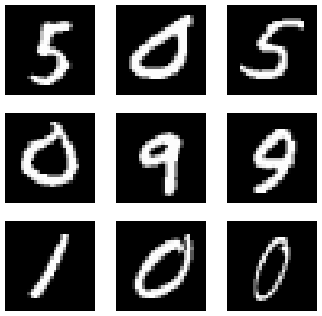
데이터가 잘 받아졌는지 확인하기 위해 9개만 출력해보겠습니다.
1
2
3
4
5
6
7
8
9
10
# 랜덤으로 9개만 시각화
figure = plt.figure(figsize=(8, 8))
cols, rows = 3, 3
for i in range(1, cols * rows + 1):
    sample_idx = torch.randint(len(mnist_train), size=(1,)).item()
    img, label = mnist_train[sample_idx]
    figure.add_subplot(rows, cols, i)
    plt.axis("off") # x축, y축 안보이게 설정
    plt.imshow(img.squeeze(), cmap="gray")
plt.show()
데이터 로더
1
2
3
4
# 데이터 로더
data_loader = torch.utils.data.DataLoader(dataset=mnist_train, # 훈련용 데이터 로딩
                                          batch_size=batch_size,
                                          shuffle=True) # 에폭마다 데이터 섞기
모델 정의하기
1
2
3
4
5
6
7
8
9
10
11
12
13
14
15
16
17
18
19
20
21
# Discriminator
D = nn.Sequential(
    nn.Linear(image_size, hidden_size),
    nn.LeakyReLU(0.2),
    nn.Linear(hidden_size, hidden_size),
    nn.LeakyReLU(0.2),
    nn.Linear(hidden_size, 1),
    nn.Sigmoid()) # Binary Cross Entropy loss 를 사용할 것이기에 sigmoid 사용!

# Generator
G = nn.Sequential(
    nn.Linear(latent_size, hidden_size),
    nn.ReLU(),
    nn.Linear(hidden_size, hidden_size),
    nn.ReLU(),
    nn.Linear(hidden_size, image_size),
    nn.Tanh())

# Device setting
D = D.to(device)
G = G.to(device)
Loss function 설정, Optimizer 설정
1
2
3
criterion = nn.BCELoss()
d_optimizer = torch.optim.Adam(D.parameters(), lr=0.0002)
g_optimizer = torch.optim.Adam(G.parameters(), lr=0.0002)
모델 훈련
1
2
3
4
5
6
7
8
9
10
11
12
13
14
15
16
17
18
19
20
21
22
23
24
25
26
27
28
29
30
31
32
33
34
35
36
37
38
39
40
41
42
43
44
45
46
47
48
49
50
51
52
53
54
55
56
57
58
59
60
61
62
63
64
65
66
67
68
69
dx_epoch = []
dgx_epoch = []
total_step = len(data_loader)
for epoch in range(num_epochs):
    for i, (images, _) in enumerate(data_loader):
        images = images.reshape(batch_size, -1).to(device)

        # Create the labels which are later used as input for the BCE loss
        real_labels = torch.ones(batch_size, 1).to(device)
        fake_labels = torch.zeros(batch_size, 1).to(device)

        # ================================================================== #
        #                      Train the discriminator                       #
        # ================================================================== #

        # Compute BCE_Loss using real images where BCE_Loss(x, y): - y * log(D(x)) - (1-y) * log(1 - D(x))
        # Second term of the loss is always zero since real_labels == 1
        outputs = D(images)
        d_loss_real = criterion(outputs, real_labels)
        real_score = outputs

        # Compute BCELoss using fake images
        # First term of the loss is always zero since fake_labels == 0
        z = torch.randn(batch_size, latent_size).to(device)
        fake_images = G(z)
        outputs = D(fake_images)
        d_loss_fake = criterion(outputs, fake_labels)
        fake_score = outputs

        # Backprop and optimize
        d_loss = d_loss_real + d_loss_fake
        reset_grad()
        d_loss.backward()
        d_optimizer.step()

        # ================================================================== #
        #                        Train the generator                         #
        # ================================================================== #

        # Compute loss with fake images
        z = torch.randn(batch_size, latent_size).to(device)
        fake_images = G(z)
        outputs = D(fake_images)

        g_loss = criterion(outputs, real_labels)

        # Backprop and optimize
        reset_grad()
        g_loss.backward()
        g_optimizer.step()

        if (i+1) % 200 == 0:
            print('Epoch [{}/{}], Step [{}/{}], d_loss: {:.4f}, g_loss: {:.4f}, D(x): {:.2f}, D(G(z)): {:.2f}'
                  .format(epoch, num_epochs, i+1, total_step, d_loss.item(), g_loss.item(),
                          real_score.mean().item(), fake_score.mean().item()))
    dx_epoch.append(real_score.mean().item())
    dgx_epoch.append(fake_score.mean().item())
    # real image 저장
    if (epoch+1) == 1:
        images = images.reshape(images.size(0), 1, 28, 28)
        save_image(denorm(images), os.path.join(sample_dir, 'real_images.png'))

    # 생성된 이미지 저장
    fake_images = fake_images.reshape(fake_images.size(0), 1, 28, 28)
    save_image(denorm(fake_images), os.path.join(sample_dir, 'fake_images-{}.png'.format(epoch+1)))

# 생성자, 판별자 각각 모델 저장
torch.save(G.state_dict(), 'G.ckpt')
torch.save(D.state_dict(), 'D.ckpt')
결과 확인
1
2
3
4
5
6
7
8
plt.figure(figsize = (12, 8))
plt.xlabel('epoch')
plt.ylabel('score')
x = np.arange(num_epochs)
plt.plot(x, dx_epoch, 'g', label='D(x)')
plt.plot(x, dgx_epoch, 'b', label='D(G(z))')
plt.legend()
plt.show()
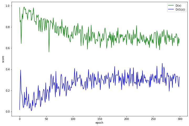
결론
결과 확인 이미지를 보면, 두개의 Loss가 0.5 로 수렴하는걸 볼 수 있다.
Reference
https://github.com/yunjey/pytorch-tutorial/tree/master/tutorials/03-advanced/generative_adversarial_network - 최윤제님 github